Game Probability Profile – Crusaders v Blues

It has been a while since my last post which dealt with Game Probability Profiles (GPP’s). Part of the reason for this is that I found the concept of the GPP to be so useful in analysing matches that I’ve been spending some time developing an application which allows for easy production of the GPP of a match in realtime. As part of this I have also added the ability to easily calculate the profiles for mismatched teams, as well as some other useful information.

To demonstrate, I will go over some key aspects of the previous weekends clash in Super Rugby between the Crusaders and the Blues.

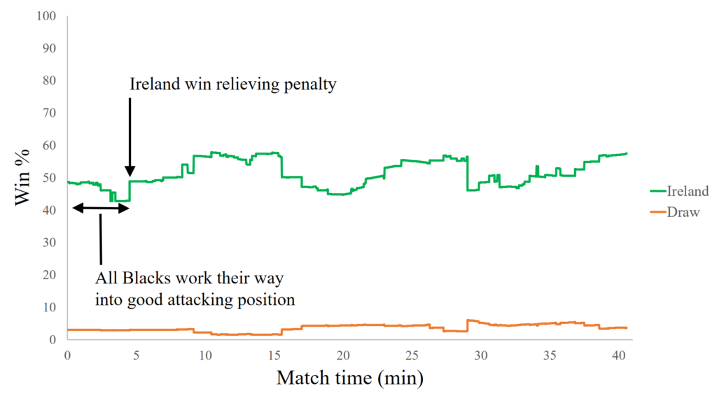
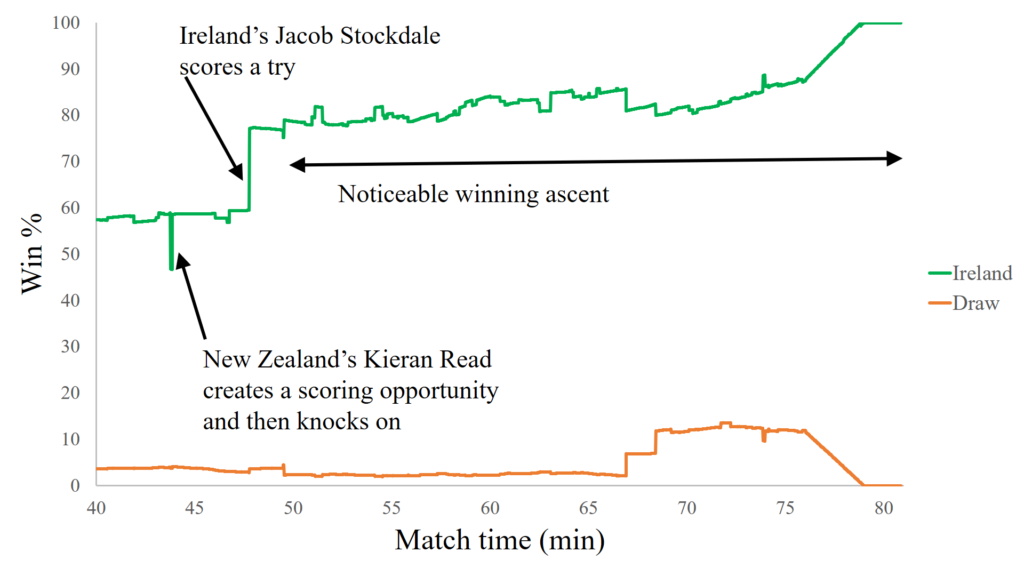
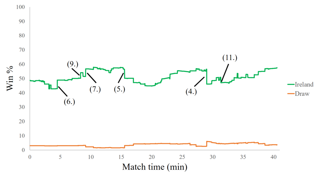
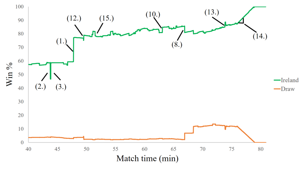
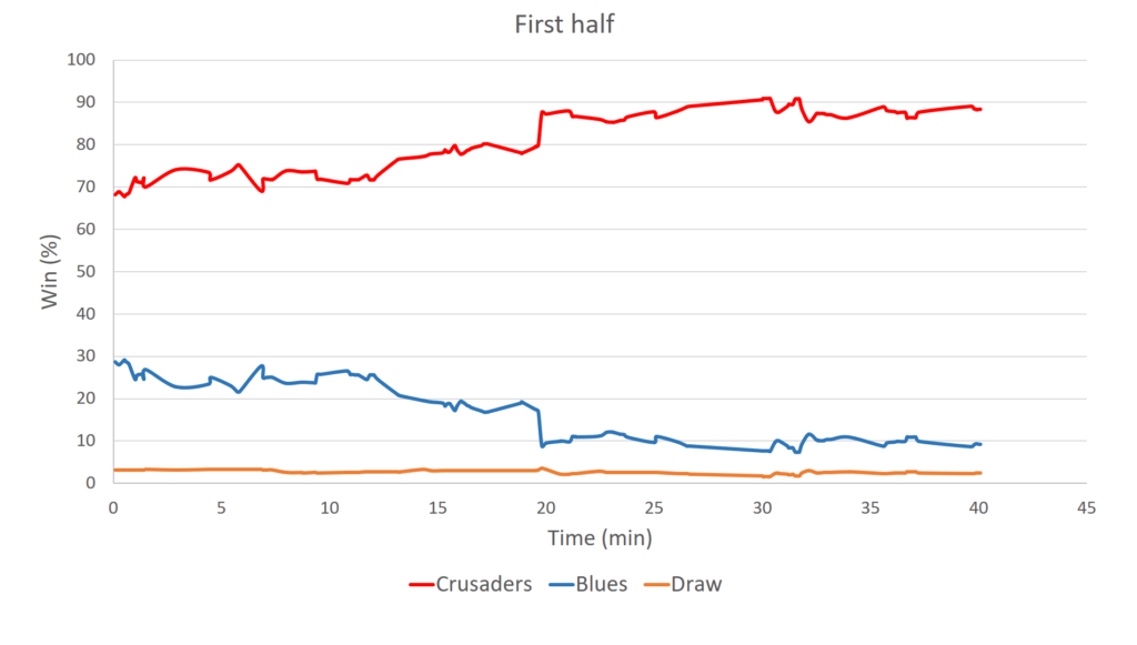
You may recall, that in the previous GPP post we looked at a match between Ireland and New Zealand, and we assumed that on that day they were evenly matched. Although this is clearly not the case for the Crusaders and the Blues, with the Crusaders being a far superior side, let’s have a look first at what the GPP would look like if they were evenly matched.

First half Game Probability Profile assuming evenly matched sides.
2nd half Game Probability Profile assuming evenly matched sides.

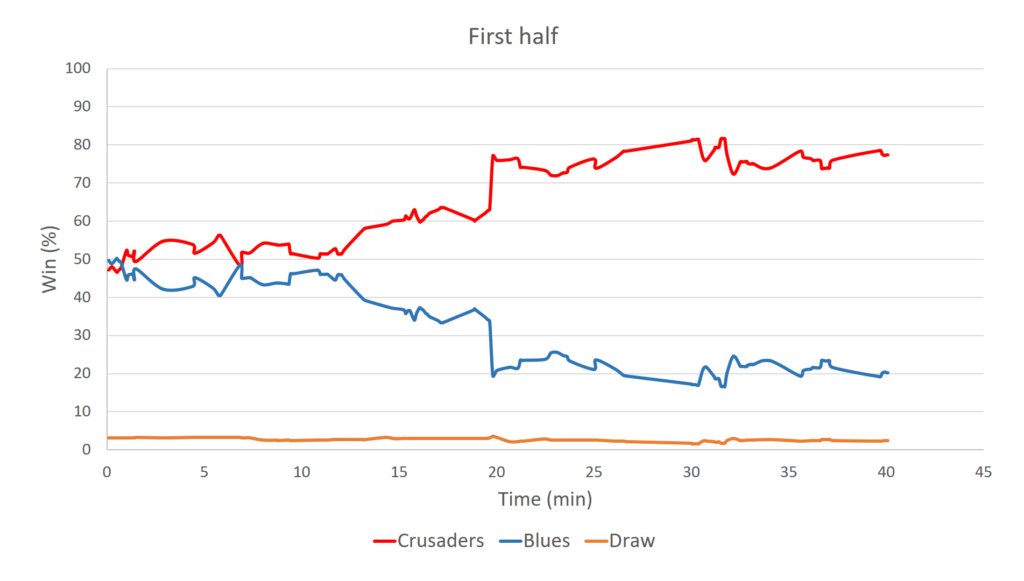
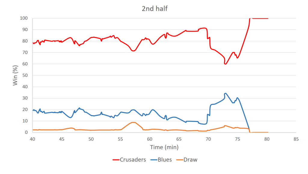
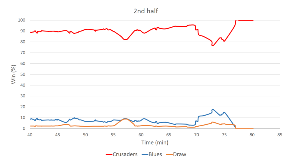
You can see that even when we assume the sides are evenly matched the GPP paints a bleak picture for the Blues. The Crusaders quickly manipulate the match into a situation where after 20 minutes they have around an 80% chance of winning. They then hold this position for most of the match, with the Blues making a late charge at the end, which on this occasion turns out to be in vain.

The winning minutes, which are a reflection of the time each team spent in a position to win the match reflect the Crusaders dominance. These were 59 winning minutes to the Crusaders, 19 to the Blues and 2 to the draw.

Time to introduce a new, very valuable statistic, scoreless winning minutes. Scoreless winning minutes are simply the winning minutes of a game calculated with all the scoring plays removed. They therefore give an indication of the tactical dominance of each side, especially when calculated under the assumption of equal winning probability. They are useful because on a given day a team might play well and put itself in good positions to score points, but not convert those opportunities. This will be reflected in scoreless winning minutes and provides the team and coach an opportunity to assess their ability to put themselves in scoring positions and deny their opponent opportunities to score, regardless of whether they managed to execute on the day. In this game under the assumption of equal winning probability the Crusaders had 39 scoreless winning minutes, the Blues 36 and 5 went to the draw. So, the Crusaders were tactically superior, and this is perhaps one of the reasons for their success. The magnitude of difference in scoreless winning minutes between the side is not particularly large, being only 3. However, the matches I have analysed to date would suggest that even a small difference like this is a good indication of tactical dominance. As I analyse more matches it will become clearer what a typical difference is and how this relates to the degree of tactical dominance.

One other interesting statistic that can be easily calculated as part of the GPP calculations is the probability that the losing side would lose by this amount or more if it were of equal quality to its opponent. For this particular game the probability the Blues would lose by the amount they did or more if they were the equal of the Crusaders is 33.8%. This goes to show that when playing an evenly matched team you can expect to lose, and sometimes by substantial margins. So, unless you have good reason to believe you are inferior, their might be no need to panic.

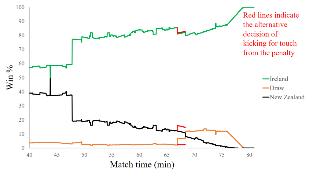
Of course, in the case of the Blues we have good reason to believe they are an inferior side compared to the Crusaders. The evidence for this comes from a comparison of their performances to date so far this season. Most notably the Crusaders have scored an average of 32.1 points per game compared to the Blues 21.8, and have conceded only 17.2 points per game compared with the Blues 22.5. And although I won’t go into the details here, it is by utilizing this information that we can calculate the actual GPP for this match which takes into account the mismatching of the sides. This is presented below.

First half Game Probability Profile.
2nd half Game Probability Profile.

We see that things look even worse for the Blues. They start out the game with less than a 30% chance of winning. This is quickly whittled down to around 10% where it remains for most of the game, except for a brief spike at the end. The winning minutes are 69 to the Crusaders, 9 to the Blues and 2 to the draw.

So, are the Blues without hope when they come up against the Crusaders?

Well, yes and no. It is true that in order to win more often they will likely need better players and tactics, such that their attack and defense are better from the outset. Doing this will minimise the winning probability deficit between them and the Crusaders from the get go.

But obviously for now they are somewhat stuck with what they have. So accepting this, there is still much they can learn from the GPP and improve their chances after the game kicks off. Let’s have a look at a couple of examples.

In the graph below we have zoomed in on the GPP from minute 16 to 17 and are displaying the Blues probability of winning the game.

Game Probability Profile segment showing the Blues losing a kicking battle.

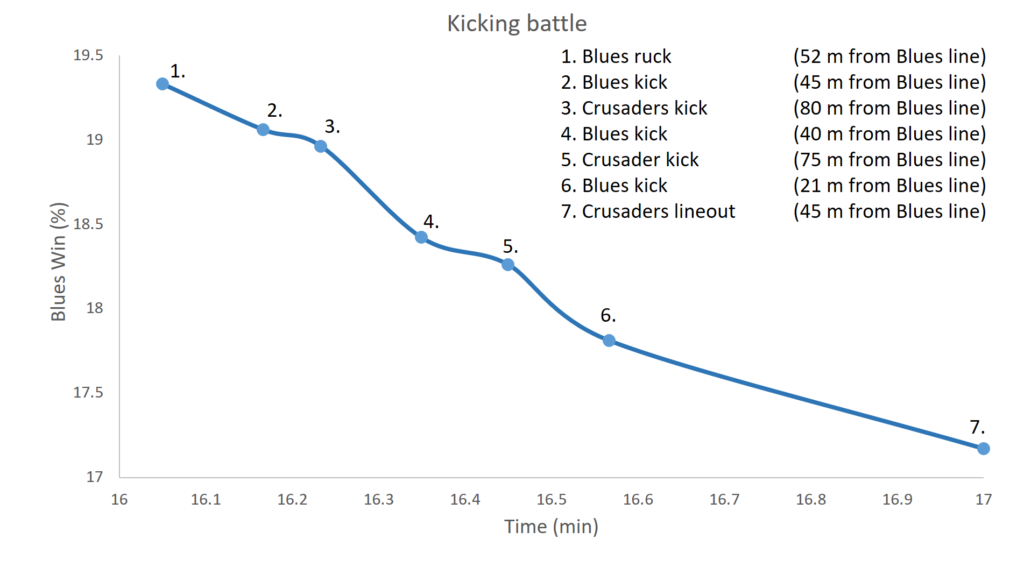
The graph shows the Blues start out with the ball at a ruck just over halfway. They then choose to engage in a territorial kicking battle with the Crusaders. With every action in this kicking battle, the Blues end up in a worse position. The end result is ultimately that they started with the ball 52 m from their own line and end up handing it over to the Crusaders 55 m out from their line (45 m from the Blues line). In the process they reduced their chances of the winning by over 2%.

Now, for us looking at the GPP it is clear and obvious that this was poor tactical play. It obviously wasn’t clear to the Blues, since they initiated this play and continued to engage in it. This demonstrates that through careful study of the GPP the Blues would be able to improve their chances to win and become better equipped to avoid situations like this. This also serves to illustrate that it is not always single large turning points that swing a match, but often the culmination of many smaller decisions can also be crucial to the outcome.

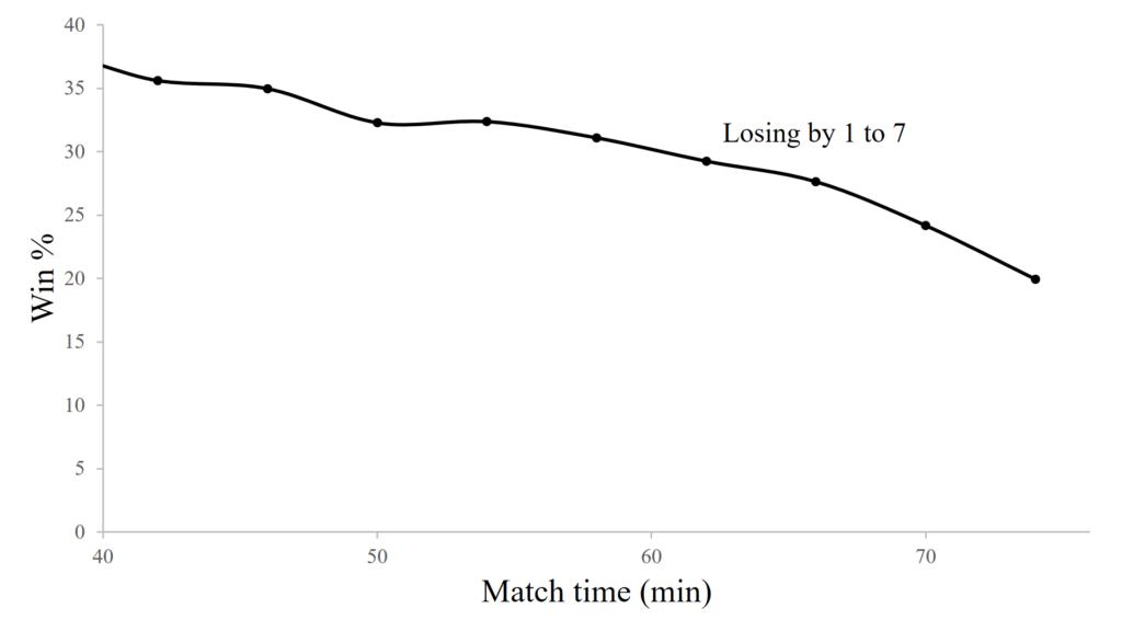
Having said that, let’s have a look at single event which has a large impact and identifies additional improvement opportunities for the Blues. The GPP segment below highlights one of the final sequences of the match. Only a few minutes remain and the Crusaders are attacking the Blues line with a lineout 20 m out. Despite this, the Blues still have a small chance of winning, around 13%. This might seem pathetic, but those who watched the match will know that the Blues fought hard as a team for this glimmer of hope. It’s around a 1 in 7 chance of winning from here, and it is better than nothing.

Game Probability Profile segment showing the result of poor discipline by the Blues late in the game.

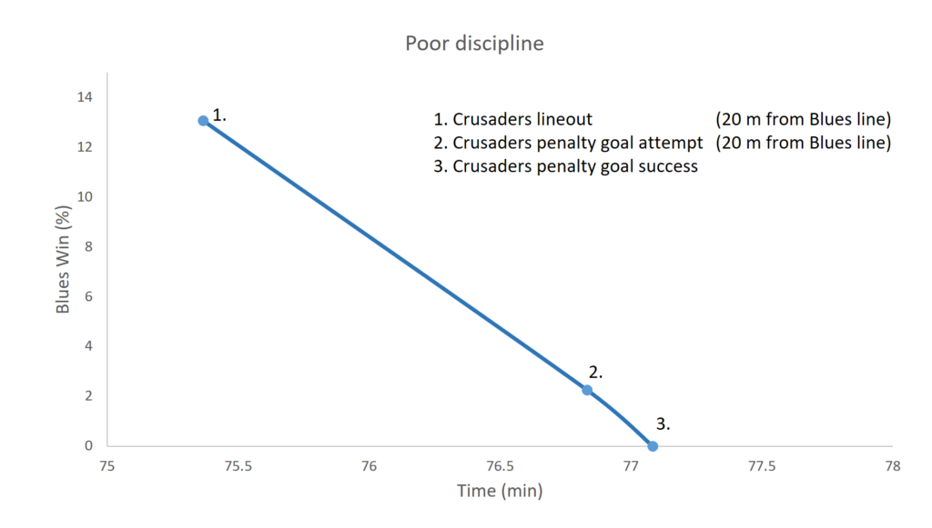
Unfortunately, at the lineout one of the Blues players gives away a needless penalty by pushing his opponent before the ball is in play. The Crusaders opt to line up a shot at goal which reduces the Blues chances to win to around 2%, and when the kick goes over their chances have reduced to 0% since there simply is no longer time left in the match for them to make up the deficit.

This is another example of something the Blues chose to do that was completely in their control. The player who gave away the penalty might have been frustrated or he may have even thought he was helping his team. I believe that if players could see the quantifiable impact of giving away needless penalties on winning percentage, then they would be less likely to give them away. The result would be improvements in their winning percentages, and obviously more wins would follow in the long term.

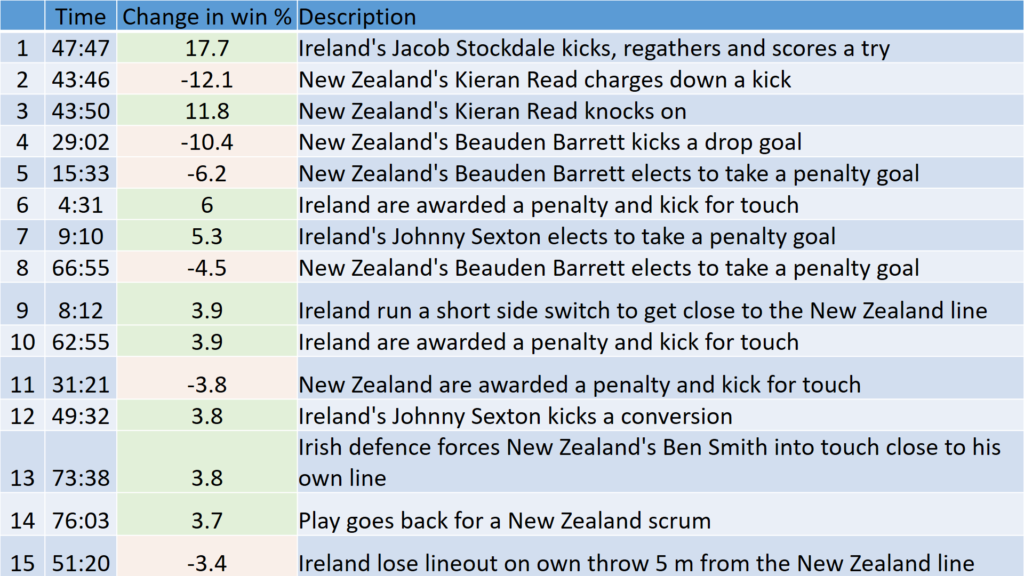
This might seem a little trivial to some. However, the GPP calculations allow us to easily rank all the turning points (winning probability swings in a match) and see what has the biggest impact. Doing this it becomes apparent that small things matter. It might surprise you to know that giving away the penalty discussed above was the single biggest reduction in the Blues winning percentage, causing a bigger reduction than the try they conceded which was the second biggest reduction from the Blues perspective. Third, was a simple handling error at a ruck in the 74th minute.

Small things matter. The Crusaders know it. Teams like the Blues need to learn it too. That’s what it takes to compete with the big boys.

There are of course many other improvements the Blues could make (as could the Crusaders) through careful analysis of the GPP calculations. In the next post we’ll examine something else the numbers tell us the Blues should be doing when they come up against superior sides like the Crusaders.

Game Probability Profiles

In the previous post we saw how Monte Carlo simulation can be applied to determine the impact of refereeing decisions on a team’s chances of winning.

This approach need not be restricted to refereeing decisions. It can be applied to any and all events that occur during the course of a contest. When this is done we end up with a Game Probability Profile (GPP), which paints a complete picture of the ebbs and flows of the chances of a team winning over the entire course of the contest.

It’s an extremely powerful tool which is useful for fans, coaches, analysts, and of course, in a gambling context. Basically anyone with a vested interest in a sport can derive great utility from a GPP. In this post we will focus on its use as a coaching and match analysis tool.

At a high level a GPP is useful to provide a complete, concise and elegant description of a game. At lower levels, its respectful study reveals the key turning points in a match and can be used to determine the strategies which contributed to the winning or losing of the match. In this article we will explore these various levels of a GPP by examining the profile of the recent Irish defeat of the All Blacks in Dublin.

The figures below show the GPP from an Irish perspective for the first and second halves of the match. To illustrate the descriptive nature of a GPP some key features have been highlighted. Note that we are assuming the teams were evenly matched to begin with. Probably a reasonable assumption in this case, but we can just as easily apply the same approach to mismatched teams in the future.

1st half Game Probability Profile (GPP)
2nd half Game Probability Profile (GPP)

The GPP shows the All Blacks started the match well, as indicated by the decline in Ireland’s winning probability during the opening 4 minutes. They controlled territory and possession and worked their way into a position in which they had attacking rucks near Ireland’s goal line. This pressure was relieved by the spike in winning probability mid-way through the 4th minute when Ireland won a penalty at the ruck. The remainder of the first half results in various back and forth flows in winning probability, which we will discuss further when we consider turning points below. For now we will have a look at the illustrative features highlighted in the second half GPP above.

Firstly, there is the large down and up spike in winning probability around 43:45. This is when New Zealand’s Kieran Read charges down a kick from Ireland’s Jacob Stockdale to create a high probability scoring opportunity, but subsequently produces a handling error which took that opportunity away. A few minutes later the biggest turning point in the match occurs when Stockdale kicks and regathers to score what would be the only try of the match. This triggers an important phenomenon, the beginning of an increasingly rapid winning ascent (or losing descent). A winning ascent occurs as the result of a side being ahead and time running out on the clock. The more a team is ahead and the less time there is remaining, the steeper the ascent. It can serve as an important trigger for the losing side to know when to switch to increasingly higher risk-reward strategies. The fact that a GPP can be calculated in real-time means that this is one useful way a coach can utilise this tool during the match (we’ll see other examples of this below where the GPP would have been useful to assist in real-time decisions like whether or not to take a shot at goal). In this particular match, the noticeable winning ascent which begins after the Irish try is scored is briefly reduced by New Zealand around the 65th minute when they kick a penalty goal, before its steepness increases around the 75th minute as the clock runs toward full time.

Before looking at some of the finer details of a GPP, we will complete our high level overview by introducing the concept of winning minutes. Winning minutes are the area under the GPP. They tell us, out of the total time in the match, how much was dominated by each team in terms of the opportunity to win. The figure below displays the winning minutes for each team for both halves of the game, as well as for the entire match.

Winning minutes for the first half, second half and overall.

Overall, Ireland dominated the winning minutes with 53.1 minutes (65%) to New Zealand’s 24.9 minutes (31%), with the remaining minutes going to the draw. The first half winning minutes were closer with Ireland having 20.8 minutes (51%) to New Zealand’s 18.3 minutes (45%), but in the second half Ireland almost completely shut New Zealand down by collecting 32.3 winning minutes (79%) to New Zealand’s 6.6 minutes (16%).

Why is this important?

Winning minutes are very useful, because in a single descriptive statistic they tell us which team created the most opportunity to win the match. This can be very important, since it removes us from focusing on the score (or other statistics which might lead us astray). The team that consistently dominates winning minutes will win more matches. So by focusing on winning minutes we are more easily able to determine when we played well, even if we went on to lose. Likewise, we can more easily tell when we played poorly, even if we went on to win (notwithstanding the usual caveats with regard to sample size).

Perhaps we are testing a new strategy and have lost a few games. It would be easy to abandon this strategy. But if it has led to a relative increase in winning minutes we might think twice before throwing the baby out with the bath water. Conversely, we could win a few matches with our new strategy but experience a relative decrease in winning minutes. Perhaps we have just been lucky, and it might be best to abandon the strategy.

Whatever the case, the key point is that if a team  consistently dominates winning minutes, the scoreboard will take care of itself in the long run.

With an understanding of winning minutes, let’s now move down a level and consider how the finer detail of the GPP can tell us not only who created the most winning opportunities, but how they were created. With that in mind, let’s take a look at the largest 15 turning points in the match. In the last post we considered a turning point to be any event which causes a significant swing in the probability of a team winning a match. We will look at the turning points from Ireland’s perspective. So, a positive turning point value represents an increase in their probability of winning, and a negative one a decrease.

15 biggest turning points.
1st half GPP with selected turning points.
2nd half GPP with selected turning points.

The largest turning point was the try scored by Ireland’s Jacob Stockdale, followed by Kieran Read’s charge down, and subsequent knock on. These are probably in agreement with the intuition of anyone who watched the match. They felt like important moments.

Of the remaining turning points on the list, only two are actually acts of scoring points. These are the Barrett drop goal and the Sexton conversion. The shot’s at penalty goal do not appear, but rather the decision to take them is the larger turning point. This is because the penalty shots carried a probability of success greater than 50%, and hence there is more value in electing to take them than when they actually go through the posts (if they go through the posts). The reverse is true of the drop goal and conversion taken in this match which were considered to have less than 50% chance of going over (the conversion was close to the sideline).

The remaining items on the list feature, among other events, relieving penalties when defending one’s own goal line, and losing one’s own lineout throw when in good attacking position. It’s also fascinating that a GPP picks up items like the effectiveness of Ireland’s blind side switch play (item no. 9) in penetrating the New Zealand defense and leading to good attacking opportunity.

It is very important to note that while we are looking at the largest turning points for illustrative purposes, this does not mean they are necessarily the most important. The cumulative sum of many smaller turning points can also lead to the creation of substantial opportunity (winning minutes) during the course of a match. This is something we will explore further in a future post.

One other really interesting item on the list is at 76:03 (no. 14), when play goes back for a New Zealand scrum resulting in an increase in Ireland’s winning percentage of 3.7%. This doesn’t register as a spike, but is the result of the time wasted setting a scrum while Ireland are in a steep winning ascent and New Zealand in a steep losing descent. What happens here is that the referee starts playing a knock on advantage to New Zealand and they use it as an opportunity to try an attacking kick, knowing that if it doesn’t come off they will still retain possession through a scrum. Players often use this tactic. The GPP shows that when you are in the middle of a losing decent, it may not be a good idea to use this tactic.

To know for sure whether it was a good idea to choose to attempt any particular action during a match, we need to compare its possible outcomes with the outcomes of alternative actions weighted by their relative probabilities of success.  This directs us to the final level of GPP analysis we will consider in this post. Namely, a ‘What-If’ analysis. As the name implies, this involves taking an event in the match and changing it to something different to see what the impact on winning probability is.

To illustrate this we’ll have a look at the decision in the match where New Zealand elected to kick a goal at 66:55. What if they had instead opted to kick for touch and take a lineout 10 m out or less from the Irish goal line? The figure below answers this question.

2nd half GPP showing the impact of an alternative decision to kick to touch instead of for goal from the penalty.

The red lines in the figure represent the change that would have occurred to the win and draw percentages if New Zealand elected to kick for touch, with the remainder of the figure simply being a replication of what actually happened in the match, as per the other GPP’s presented above. The result shows that the decision has about the same impact either way on Ireland’s chances of winning. The decision to kick a goal, increases New Zealand’s chances of a draw by about 5% but has virtually no impact on their chances of winning. This is because it still leaves them requiring two scores to win. On the other hand, had they kicked for touch, their chance of a draw remains almost unchanged, but their chance of winning increases by 4%. In this particular case, in terms of winning the game it is more valuable to have a relatively small chance of scoring a try than a good chance of scoring a penalty goal. So, if the All Blacks were trying to win the game, they made the wrong decision. If they were trying to draw it, they made the correct decision.

This is contrary to some conventional opinions which suggests it is always better to take the shot at goal. Indeed it’s a simple mathematical exercise which I’ll go over in another post to show that in many cases this is true. However, this standard approach often only considers the quality of the kicker in the calculation. In doing so, it neglects the fact that the current score, time remaining in the match, location of the kick at goal, and relative mismatching of the teams are important considerations in this calculation too. The GPP incorporates all of these factors and therefore comes out with the correct decision where the conventional simple calculation would produce an incorrect decision.

One final thing to note on the figure above is the downward slope on the red line of New Zealand’s winning percentage after they hypothetically elect to take the lineout. This indicates that not only should New Zealand take the lineout if they want to win, but they should take it as quickly as possible. Ireland on the other hand should take as much time as possible forming the lineout, as indicated by their upward sloping red line. In this regard the GPP can not only help us to make the correct decision, but serve as a reminder to the pace of play we should adopt once it becomes an important factor.

We need not restrict ourselves to examining decisions around shot’s at goal. We have already seen above that New Zealand’s decision to try an attacking kick in general play when they had a knock on advantage may have been questionable.  What about other events? For example, should a team have kicked or kept the ball in hand in a other situations? If they should kick, what location should they kick too? Indeed, we can look at all events in the game when performing a What-If analysis. Doing this actually reveals the general strategy that Ireland uses to gain advantage by maximising opportunities (winning minutes). It’s interesting enough that we’ll leave this analysis for another post.

For now we’ve made good progress in introducing the GPP and seeing that it is an extremely valuable tool for enabling us to focus on what is important to our chances of winning. It’s fascinating that in some cases it confirms our intuition and in others challenges it, revealing new knowledge in the process. It can form an important loop of assisting real-time match decisions, post-match analysis, and subsequent design of strategies for upcoming matches. The bottom line is that teams who exploit the information contained in a GPP will win more games. In future posts we’ll look to delve deeper into this interesting area.

Can a referee cost a team a win?

Complaining about the performance of the referee goes hand in hand with sporting contests. It’s currently very topical in the rugby world, as in the weekend just past a controversial referring decision denied England a try against the All Blacks late in the game. This has many, especially some in the English media, claiming the referee cost England the game.

It seems like a good time then for us to answer the age old question, can a referee cost a team a win?

We’ve all heard people claim that the referee cost their team the game. We’ve probably all also heard the extra qualification that is sometimes added, that a referee can cost a team the game, but only if they lose by less points than the decision cost them.

An example of this type of thinking comes from the coach of the Australian national rugby team, Michael Cheika.

“We can only call it a turning point if we lose by less than one score, prehaps?” Michael Cheika

Cheika is referring to a decision that cost his team, the Wallabies, a try. The Wallabies then went on to be well beaten by more than a try in that game, and as a result Cheika feels he can’t call this a turning point. But if they had of lost by a try or less, he would presumably be comfortable with calling it a turning point.

Now I can’t be sure what Michael Cheika intended by a turning point, but in this post we need an objective definition of a turning point. We’ll assume that in a sporting contest a turning point is a significant shift in the probability of winning from one team to another (apologies if that’s not what you meant coach Cheika).

So let’s consider not only the question of whether or not a referee can cost a team a game, but also whether or not they can only cry foul if they lose by less than the decision cost them.

To answer these questions we don’t actually need to do any calculations or simulations. The question can be answered with a conceptual understanding of probability. However, we will use a simulation based approach as it will help guide us toward this understanding in a more visual way.

Note that we’ll be assuming that the refereeing decisions we discuss here were incorrect. Whether they were or not is a debate for another day. The simulation results presented will also be for matches between two evenly matched professional level teams. By extension we will also be assuming any real world games discussed below were between relatively evenly matched teams. This might be a stretch in some cases, but it doesn’t detract from the points we are trying to illustrate here. In the future we will look at simulations between teams with varying degrees of mismatching. Finally, we will restrict ourselves here to considering situations where we assume an incorrect referring decision almost immediately resulted in the scoring of points which we assume to be attributable to the decision.

With that said, let’s get to it.

The graph below was composed from 5000 Monte Carlo simulations of full rugby matches. It shows the probability of going on to win a game when trailing by 1 to 7 points from the 40th to the 76th minute of the match.

Probability of winning when trailing by 1 to 7. Values calculated by counting values in bin widths of 4 min from 5000 Monte Carlo simulations. Data points are plotted at the center of the time range of each bin.

The graph shows that at the beginning of the half being behind by 1 to 7 drops a teams chances of winning the match to about 35%. From there the chances of winning decline as the match progresses. This decline becomes noticeably steeper as the final 15 minutes of the match are entered. This probability will tend to zero as the final whistle approaches. But in a one score game, it will never quite get there. There will always be hope as long as there is time on the clock.

Note, that if we did more simulations the trend in the graph would likely be smoother, and the values more precise. As it stands they should be considered to have a precision of about plus or minus 3%.

Now, from this position of losing by 1 to 7 points, let’s assume that a bad refereeing decision directly results in a try scored by our opponents under the posts, so that the conversion is assumed a formality. We go down by an additional 7 points, and now move to the category of losing by 8 to 14 points. The graph below shows this transition.

Probability of winning when trailing by 1 to 7 and 8 to 14. Values calculated by counting values in bin widths of 4 min from 5000 Monte Carlo simulations. Data points are plotted at the center of the time range of each bin.

The trend in the graph remains similar, but it shifts down considerably, a clear turning point. In fact it shifts down by a fairly consistent margin of about 20% at all time values. So, a bad refereeing call which results in 7 points against us in the second half when we are already trailing by 1 to 7, reduces our chances of winning by about 20%. If this bad call occurs at the beginning of the half, our chances of winning drop to about 18%. But if it occurs around the 76th minute, they are reduced to around 1%.

Let’s go one final step further, by considering the impact of a bad call which transitions a team already losing by 8 to 14 to losing by 15 to 21. This is shown  in the graph below.

Probability of winning when trailing by 8 to 14 and 15 to 21. Values calculated by counting values in bin widths of 4 min from 5000 Monte Carlo simulations. Data points are plotted at the center of the time range of each bin.

We see that the bad decision early in the half drops our chances of winning from about 18% to around 8%. Late in the half they drop from around 1% to pretty much 0%. A drop to 0% will occur whenever it is not practically possible for us to win the game in the time remaining.

This analysis allows us to make three important statements about the impact of poor refereeing decisions of the type we are considering, and in doing so answers our question of whether or not the referee can cost us the game.

1. Reducing the probability of winning – the most common result of a bad decision is to reduce the probability of winning, but still leave us with a chance to win the game.

2. Denying the opportunity to win – the reduction in the probability of winning can result in it becoming zero. This occurs when there is not sufficient time left in the match to score the points required to win. In this case the referee has denied us the opportunity to win. This is subtly different from costing us the game, since if the decision had not been made both teams would still have a chance to win and therefore we can’t be sure we would have won.

3. Costing the game – if a refereeing decision denies us the chance to put our opponent in a position in which their probability of winning would be reduced to zero, and they then go onto win the match, that decision will have categorically cost us a win.

So the referee can cost us the game.

What about the idea that a referee can only cost a team the game if they lose by less points than the decision cost their team?

Well, interestingly there is some truth to this.

Consider the situation where the criteria for costing a game is met as specified above. A team needs $latex x$ scores to give them the win, which will put them a single score ahead of their opposition. There isn’t time for $latex x + 1$ scores. So if the team who is $latex x$ scores ahead is denied an opportunity to go $latex x + 1$ scores ahead due to a poor refereeing decision, and their opponent then goes onto win, it can only be by scoring $latex x$ times, since that is all their is time for. They will win be one score (or less in a multipoint scoring system).

Notice I said there is some truth to this. That’s because there can be many situations where a refereeing decision will cost a team a given amount of points and they then go onto lose by less than that amount, but the criteria for costing the game will not be met. For example, we saw earlier that at the beginning of the half when we are trailing by 1 to 7 a bad decision which results in a try against us reduces our chances of winning to 18%. We still have a chance to win, so even if we go onto lose by less that the bad decision cost us, we can’t claim it cost us the game. So, while a team who has been cost the game will lose by less than the decision cost them, losing by less than a decision cost a team does not guarantee they were cost the game.

What about a turning point? Do we have to lose by less than the amount a bad call cost us in order to consider ourselves disadvantaged by the decision. In terms of a turning point, which we consider to be a swing in the probability of winning, the answer is obviously, no. We have seen a bad refereeing call can result in a large drop in the probability of winning, regardless of what happens next. The final score is irrelevant. Likewise, the referee can deny us the opportunity to win without the final score having any relevance.

In fact, in a sport like rugby, large turning points will be by far the most common way a poor refereeing decision will impact a team. Being denied the opportunity to win will be less common, and being cost the game even less common again. So when we fixate on decisions where a team may have been cost the game, or very nearly so, we miss out on identifying many other opportunities for refereeing improvement.

In my opinion, we should be focusing on turning points. They are much more common, and therefore provide many more opportunities for improvement. The situation is often made worse by the fact that teams disadvantaged by a turning point can still go onto win. Unfortunately, most teams don’t complain as loud, if at all, when they win. So a lot of opportunities to highlight and improve our refereeing slip under the radar. One of the advantages of quantifying the effect of bad calls in the way we have done here, is that they are less likely to be overlooked because we can put a value on their effect, regardless of the end result of the match.

To highlight what we have discussed, let’s have some fun by looking at how much some famous real life controversial refereeing decisions impacted the teams involved. I have prepared a look up table below to assist us, and will look at a few well known games that I found interesting (I’m a New Zealander so forgive my bias selection of games involving the All Blacks). Feel free to apply the same process to any other games that interest you. Once again, treat the values as about plus or minus 3% precision (which explains why, for example, we see some small upward fluctuations when moving from one cell to the one below it).

Probabilities of winning (%) when losing or winning by various margins at different times in the match. L = Losing, W = Winning, D = Draw.

Match 1 – New Zealand 37 Australia 10 – October 18 2016 Eden Park, Auckland.

This is the game Michael Cheika was referring to in the quote at the beginning of this article. With about 45 minutes on the game clock the Wallabies were trailing by 15 to 10 when Henry Speight scored a try which would subsequently be disallowed to the dismay of many.

Using the table above the Wallabies had a 32.4% chance of winning (Row >44 to <= 48, Column L 4-6), and were denied the opportunity to move to a 51.6% chance of winning (Row >44 to <= 48, Column D/W 0-3). In making his decision the referee reduced the Wallabies chances of winning by 19.2%.

The decision did not cost the game, and it did not deny the opportunity to win. It did result in a major turning point, which disadvantaged the Wallabies. By focusing on whether or not they lost by less than the decision cost them, coach Cheika and the Wallabies missed the opportunity to identify a crucial turning point. The failure to highlight this makes it less likely that an opportunity for refereeing improvement was identified and subsequent action taken (action is always more likely when people complain).

Match 2 – England 15 New Zealand 16 – November 10 2018, Twickenham.

At the time of writing, this game occurred in the weekend just past. With about 75 minutes on the game clock England were trailing by 15 to 16 when Sam Underhill scored a try which would subsequently be disallowed due to an offside infringement.

Using the table above England had a 28.2% chance of winning (Row >72 to <= 76, Column L 1-3), and were denied the opportunity to move to a 76.1% chance of winning (Row >72 to <= 76, Column W 4-6). In making his decision the referee reduced England’s chances of winning by q whopping 47.9%.

This decision is still being debated. Assuming it is incorrect, while it did not cost England the game, or deny them an opportunity to win, you can see it had a huge impact on England’s chances of winning. A very big turning point indeed.

Match 3 – France 20 New Zealand 18 – October 6 2007, Cardiff.

This game was a quarter final match in the 2007 Rugby World Cup. With just over 68 minutes on the game clock New Zealand were winning by 18 to 13 when France scored a try after a forward pass went unnoticed by the referee and his touch judges.

Using the table above New Zealand had a 72.3% chance of winning (Row >68 to <= 72, Column W 4-6), which was reduced to a 33.7% chance of winning (Row >68 to <= 72, Column L 1-3). New Zealand’s chances of winning were reduced by about 38.6%.

This game is still talked about on a regular basis in New Zealand. Just buy a New Zealander a beer, and ask him about this game. When he tells you that referee Wayne Barnes cost New Zealand the game, have some fun correcting him. Tell him New Zealand were not cost the game, or denied the opportunity to win. It was simply a turning point which reduced their chances of winning. In fact they still had about a 1 in 3 chance of winning. They just didn’t take it!

Let’s summarise.

A referee can cost a team a win. When this happens, that team will lose by a score or less. However, losing by a score or less even when a team was cost a score by a poor refereeing decision doesn’t guarantee they were cost the game.

In addition to being cost they game, a refereeing decision can also deny a team the opportunity to win. However, the most common result of a poor refereeing decision is to cause a turning point which shifts the probability of winning toward one team and away from the other. If we focus on and quantitatively understand turning points, as we have done here, we identify many more opportunities for the improvement of referee decisions in crucial situations. This in turn, provides us with more opportunities to improve the spectacle of the game for all involved.

Finally, note that although we have restricted ourselves to situations in which points were scored. We need not. In the future we could also readily determine what the effect of a incorrect decision such as a knock on call has on the probability of a team winning at various stages of the game and various locations on the field. We can also look at player decisions. For example should a player take a tackle or chip ahead in a certain situation? Should we kick for touch or take a shot at goal in a certain situation? In other words, which option will maximise our chances of winning?

How much does size matter in rugby?

We all know size matters in rugby. In fact it’s a big part of what makes the sport such a spectacle. There’s something primal about high speed collisions.

But how much does size matter? How important is it to winning a rugby game?

With the next Rugby World Cup rapidly approaching, we’ll try and answer this question by taking a look back to the very first Rugby World Cup which took place in New Zealand in 1987.

The world has changed a lot since 1987, and the size of rugby players is no exception. To see how this has affected the game, we will take the world cup winning All Black teams from both 1987 and 2015 and play them against each other in 2000 Monte Carlo simulations. For those looking for an explanation of how such simulations work, refer back to the first post.

Because we are interested only in the effects of size (height and weight), we’ll give  all the players equal skills (e.g. handling and tackling) and physical abilities (e.g. speed and acceleration), but allow their height and weight to be set to their actual values. For simplicity, their equal skills and physical abilities will be set at the level of a typical modern day rugby player in each position, since we already have reasonable input data for this.

The table below presents the starting lineups, including a comparison of the heights and weights of the 1987 and 2015 All Black sides. The bracketed values give the relative increase or decrease of the 2015 side over the 1987 side.

Comparison of the heights and weights of the starting lineups of the 1987 and 2015 Rugby World Cup winning teams.
 1987Height
(cm)
Weight
(kg)
2015Height
(cm)
Weight
(kg)
1Steve
McDowall
182102Joe
Moody
188
(+6)
120
(+18)
2Sean
Fitzpatrick
183105Dane
Coles
184
(+1)
108
(+3)
3John
Drake
18399Owen
Franks
185
(+2)
118
(+19)
4Murray
Pierce
198107Brodie
Retallick
204
(+6)
121
(+14)
5Gary
Whetton
198105Sam
Whitelock
203
(+5)
120
(+15)
6Alan
Whetton
193100Jerome
Kaino
195
(+2)
109
(+9)
7Michael
Jones
18598Richie
McCaw
187
(+2)
107
(+9)
8Wayne
Shelford
189107Kieran
Read
193
(+4)
111
(+4)
9David
Kirk
17373Aaron
Smith
169
(-4)
83
(+10)
10Grant
Fox
17572Dan
Carter
180
(+5)
92
(+20)
11Craig
Green
17879Julian
Savea
192
(+14)
103
(+24)
12Warwick
Taylor
17979Ma'a
Nonu
182
(+3)
108
(+29)
13Joe
Stanley
17883Conrad
Smith
187
(+9)
95
(+12)
14John
Kirwan
191100Nehe
Milner-Skudder
180
(-11)
90
(-10)
15John
Gallagher
19085Ben
Smith
186
(-4)
94
(+9)

On average the 2015 All Blacks are taller than their 1987 counterparts by a fairly modest 3 cm. All but three players in the 2015 side are taller than the player in the same position on the 1987 side. The biggest difference between the same position is in the left wing spot where 2015’s Julian Savea is 14 cm taller than 1987’s Craig Green.

The differences in weight are more striking.

On average the 2015 All Blacks are heavier by 12 kg. All but one player in the 2015 side is heavier than the player in the same position on the 1987 side. The biggest difference between the same position is at inside centre where 2015’s Ma’a Nonu is a whopping 29 kg heavier then 1987’s Warwick Taylor. In the fly-half position, two All Black greats square off in 2015’s Dan Carter and 1987’s Grant Fox. Carter is not considered exceptionally big in the modern game, but still weighs in 20 kg heavier than Fox.

It’s not all bad news for 1987. One player is taller and heavier than his 2015 version. All Black legend John Kirwan is 11 cm taller and 10 kg heavier than 2015’s Nehe Milner-Skudder in the right wing position. Perhaps this is part of the reason why Kirwan was so good in his era?

So, let’s run our 2000 match simulations and see how much of the size advantage of the 2015 team translates into winning advantage. The chart below presents the results.

The results show that the 2015 All Blacks win 59% of the games, 38% are won by the 1987 All Blacks, with the remaining 3% ending in draws. Two perfectly evenly matched sides will each win around 48.5% of matches, so through increased size alone the 2015 All Blacks have increased their chances of winning over 1987 side by about 10%.

So what causes this advantage? Is it the increased height, increased weight, or a combination of the two?

To answer this question we will return to running some simulations with input consistent with two evenly matched professional rugby sides. The same input used in previous posts. When doing this but allowing one team to be 10 cm taller than the other in every position and running 2000 match simulations, no significant difference in winning percentage was observed. This tells us that a typical professional rugby team is already sufficiently tall, and that height for heights sake is not of much further use to them.

Why might this be? Well, most of the aerial contests in rugby in general play involve the ball coming down from a relatively steep angle. They are contested by jumping, and it is a players ability to jump high rather than be tall that is important in these contests. Tall players might be more useful in the lineout, but it would appear that a 200 cm lock is already sufficiently tall, being 210 cm tall does not appear to improve the teams chances of winning. At least not in a statistically significant way over 2000 matches.

Assuming no significant interaction between height and mass, it must be that the improvement in winning is a result of increased mass only. In this regard we note that height is still a useful attribute to a rugby team, as a large frame likely comes with more mass. We also note that mass is not important to a rugby team in and of itself. It’s when is combines with velocity to create momentum that it becomes, well, hard to stop (excuse the physics pun).

The graph below gives us a closer look at the effects of increased mass by comparing our two evenly matched rugby sides whilst allowing one of them to progressively increase the weight of every player on the team, whilst holding all of their other attributes constant. Each data point represents 2000 match simulations.

The effect of increasing player weight on the winning percentage of a typical professional rugby team.

The results show that the winning percentage increases from around 48.5% to 63% over a 20 kg range. The line is in fact highly linear ($latex R^2=0.999$), with a slope of 0.74 win percent per kg. This means that, all other things being equal, our typical professional rugby team will gain about 3/4 of a percent in winning probability for each kg in weight they gain over the range we have tested. Another way of stating this is for every 1.4 kg they gain they will increase their probability of winning by 1%. The key here is that this weight must be gained in such a way that all other things remain constant. For example, they must not lose speed, fitness or have the quality of their skill execution decline. Achieving mass gain without any such reductions will require skill on the part of the strength, conditioning, and coaching staff.

In any case, we have made an important step in this post by moving from knowing intuitively that size is important to performance in rugby, to being able to quantify its value. We have also importantly been able to prioritise mass as being more important than height. Among other explorations, we’ll continue to progress toward the goal of determining not just what is important, but how important it is. For example, we know mass is important, but is it more important the speed or handling? The answer will of course be different for different teams depending on their relative strengths and future potential, but whatever the case, determining relative importance of any parameter that is related to performance will ultimately allow us to prioritise our training efforts and maximise our chances of winning. After all, that’s what it’s all about.

If you enjoyed this post, don’t forget to subscribe by entering your email above. Feel free to share this article too.

How important is the bounce of the ball in rugby? – Part II

In part I of this post we looked at how chance plays a role in determining the result of rugby matches. We saw that no matter how well we think our team is prepared, they will sometimes suffer heavy losses against sides they are evenly matched against. A sports organisation who understands this and reacts appropriately can gain an advantage. If you haven’t already read part I, it might be a good idea to go and read it first, since in this article we will assume some of the concepts discussed in there are already understood.

In this post we will expand on the concept of how chance effects rugby games by looking at missed tackles between the same two evenly matched sides and using the same 5000 Monte Carlo match simulations presented in part I.

Let’s start by having a look at the missed tackle differential between the teams (home team missed tackles minus away team missed tackles), just as we looked at the points differential in the previous post.

We expect the mean missed tackle differential between two evenly matched sides to be zero. For our 5000 Monte Carlo simulations the mean was -0.1 with a standard deviation of 9.1. This mean is more than close enough to zero for our purposes, and we note that if we had carried out more simulations this value would have eventually converged in zero.

What would we expect the mean and standard deviation of the missed tackles of a real rugby competition to be, based on this result? Well we might expect the mean to be a little less than zero if the missed tackles are somehow involved in the hometeam advantage seen in part I, and the home team misses less tackles than the away team. We might also expect that the standard deviation will be larger since in a real competition not all matches will be played between such closely matched teams. This will result is a larger spread in missed tackles as the result of a larger skill differential between the sides, and hence a larger standard deviation. The mean and standard deviation of the missed tackle differential in the 2016 Super Rugby competition was -3.0 with a standard deviation of 11.2. As hypothesised, the mean is a little less than our simulations and the standard deviation larger, and this gives us some degree of confidence that things are as they should be.

Returning to the simulation results, by tallying up the simulation results we produce the table below which shows the probability of various missed tackle differentials from the perspective of the home team.

Probability of missing less and more tackles than the opposition for two evenly matched teams.
ResultProbability (%)
15+ less missed tackles than opposition4.3
11 to 15 less missed tackles than opposition8.5
6 to 10 less missed tackles than opposition15.0
1 to 5 less missed tackles than opposition21.1
Misses tackles equal to opposition4.5
1 to 5 more missed tackles than opposition20.1
6 to 10 more missed tackles than opposition14.3
11 to 15 more missed tackles than opposition7.6
15+ more missed tackles than opposition4.6

Let’s say that in a given match a team misses 6 more tackles than their opposition. Summing the bottom three rows of the table shows us they should expect to do this by chance 14.3 + 7.6 + 4.6 = 26.5 % of the time.

For arguments sake we’ll assume missing 6 or more tackles than our opposition would result in the coach berating his players for their poor defensive commitment and putting them through a defense focused training regime the following week, at the expense of time spent on other areas of training (since there is only so much training time available).

Is this an unjustified decision by the coach? Well, if the coach has no other valid reason to believe his defense has suddenly become worse, then it is absolutely an unjustified decision.

And this is where many people get into trouble with their thinking when making decisions like this. Their argument goes something like, ‘they defended poorly, therefore they need to train defense’. However, they only defended poorly in the misguided sense that it was not the result we hoped for. In reality, this is just a legitimate sample from the teams performance profile, or distribution of outcomes. No team or individual should be berated for producing expected samples from their distribution. To do so is nonsensical, just as it would be nonsensical to berate a coin for producing a head when we were hoping for a tail.

To try and understand this better let’s drill down a little further by looking at the individual performances in a single game where the home team missed 6 more tackles than their opposition. The table below shows the players who missed tackles in a single such game, and therefore contributed to the 6 more tackles missed than the opposition in this particular game.

Players who missed tackles on the home team in a single match in which the home team missed 6 more tackles than the away team
PositionMissed tackles
Prop3
Openside flanker3
Number eight3
Hooker2
Prop2
Blindside flanker2
Wing2
Outside center2
Lock1
Halfback1
Inside center1
Fullback1

The table shows that 12 players contributed to a total of 23 missed tackles. The average missed tackles per game for a side in the 2016 Super Rugby contest was about 20, so this team missed 3 more than average. Because we know that they missed 6 more than their opposition in this particular game, we know that the opposition must have missed three less tackles than average. The worst offenders were three players who each missed three tackles each. Let’s pick on the first player listed in the table, the prop who missed three tackles, by examining his performances a little more closely. We’ll do this by looking at the his missed tackle performance profile as represented by the probabilities in the table below calculated over the 5000 Monte Carlo simulations for which we have data on him.

Single game missed tackle probabilities calculated from 5000 Monte Carlo match simulations for the prop (jersey number 1) on the home team.
Number of missed tacklesProbability (%)
035.0
135.3
218.9
37.1
4+3.6

The table shows us that our prop is normally a pretty reliable performer missing 0 or 1 tackles in more than 70% of the matches he plays. He will miss 3 or more tackles 7.1 + 3.6 = 10.7 % of the time. So whilst the 3 tackles he missed in the particular match above are not his usual performance, they still constitute expected results from his performance distribution. Therefore, unless we have other any valid reasons to believe he might be getting worse at tackling we should probably just except that this is the result of chance. Approaching him when there is no valid reason to do so may put unnecessary strain on the player coach relationship. If he missed say 4 or more tackles in consecutive games we might be more justified in taking some action since this would only be expected to happen 0.1 % of the time (0.036 x 0.036 x 100).

As a side note it will generally be better to monitor the proportion of successful skill executions. In the case of missed tackles this would be the number of missed tackles divided by the total tackles attempted. But that is a story for another day, and does not change the point we are trying to illustrate here.

So what should you do if you want to improve your teams tackling? Obviously you should train tackling. All we are saying here is that you should not make the decision to prioritise this training based on a flawed reactive understanding of probability. We’ve all seen teams who do this. One week they need to fix their defense. The next their defense is fixed but their handling needs work. Then they aren’t fit enough. Then the defense they miraculously fixed a few weeks back, has somehow broken again, and the cycle continues. This headless chook approach to coaching is a pretty good sign of a coach with no understanding of probability. Don’t be surprised to see their team sitting closer to the bottom of the ladder.

A team that can avoid this approach, will have a better chance of getting their training priorities right just by virtue of the fact they will be less likely to overcommit training time to certain areas, and as a result neglect others. In the long term they will gain advantage over other teams employing the headless chook approach.

Just what training priorities should be is another question all together. Naturally we should focus on those things that contribute the most to winning. But what are those? How do they differ for different teams? Those are questions we will look to answer in a future article.

Finally bare in mind that although this article has used tackling as an example, the general principles obviously apply to anything we might consider training. Bare in mind also that training players in a skill will result in their distribution or performance profile for that skill changing. This then becomes the new standard which they should be evaluated against when determining whether or not their is any reason to be concerned about their recent performances.

How important is the bounce of the ball in rugby? – Part I

Bounce of the ball. Rub of the green. Chance. Whatever you want to call it, we all know it plays some kind of role in determining the outcome of our favourite sporting contests. But just how important is it? That’s the question we will answer in this article for a rugby match between two evenly matched teams.

If we think about two evenly matched teams, we all intuitively understand that each team will win 50% of the time. We don’t need any sophisticated math to tell us this. It’s a simple coin flip.

Most of us also assume that a match between two perfectly evenly matched sides will be close. But is this true? How close is close?

It’s an important question to answer, simply because the careers of coaches and players hinge on wins and losses. A big loss, or series of losses, often sees coaches fired and players dropped. On the other hand, a big win or series of wins might be enough to earn a coach or player a new contract.

Once again, we can use Monte Carlo simulation to shed light on this situation. For those looking for a brief introduction to how we are using Monte Carlo methods in a sporting context, have a read of the first post where we considered how good a rugby team where the great Jonah Lomu occupied every position might be. But for now, we’ll get right to it and carry out 5000 full rugby match simulations between two evenly matched sides playing at the professional club level.

What do we expect the mean points differential (home team score minus away team score) between the sides to be?

In the absence of any home team advantage, which our simulations assume, the answer is zero. The points difference between two evenly matched sides should always average out to zero in the long term. The mean of our 5000 Monte Carlo simulations is just that, 0.0.

The standard deviation of the points differences of our simulations is 19.8. For those not familiar with statistics, the standard deviation simply tells us how much our data is spread out around the mean. The higher the value the more it is spread away from the mean. In the case of points difference, a higher standard deviation means more games are won and lost by large margins. A lower standard deviation means more games are won or lost in closely contested matches.

What would we expect the mean and standard deviation of a real rugby competition to be based on this result? Well, we would expect the mean to be a little more than 0 (we are talking from the perspective of the home team), since home town advantage is generally considered to be a real phenomenon. We would also expect the standard deviation to be a little more than 19.8, since in real professional competitions not all games are played by evenly matched teams. When two teams meet where one is a better than the other we would expect the points differential to be on average a little more, and therefore the spread in our data, as indicated by the standard deviation, to be a little more.

The mean of the points differential of games from the 135 round robin games played in the 2016 Super Rugby contest was 4.3 with a standard deviation of 21.9. As we hypothesised, the mean and standard deviation of the real world competition are a little larger than what our Monte Carlo simulations predict for two perfectly evenly matched teams. This comparison gives us some degree of confidence in the output of our simulations.

As a side note, the difference between the mean points difference of our simulations and that of the Super Rugby data is statistically significant, which suggests home team advantage is real and worth about 4 points per game. Note also, that the distribution of points differences is also approximately normal. This is quite a useful result, but not essential to what we are trying to do here so I have discussed this a little more at the end of the article.

Let’s get back to our main objective of determining how important chance is in determining the outcome of rugby games.

We are interested in the percentage of games that fall into any given score category. We can calculate this simply by counting up how many games fall into say the win by 1 to 10 points category (from the perspective of the home team in our case). These results are shown in the table below.

Probability of losing and winning a rugby match by various margins for two evenly matched teams.
ResultProbability (%)
Loss 30+6.4
Loss 21 to 308.8
Loss 11 to 2014.4
Loss 1 to 1019.1
Draw3.0
Win 1 to 1019.0
Win 11 to 2014.1
Win 21 to 308.7
Win 30+6.5

What struck me immediately is the first entry in the table, which shows we will lose around 6.4% of games by more than 30 points. So, against a team who is our equal, chance will have us get absolutely flogged about 1 in every 15 times we meet. A 30 point drubbing is the sort of result that has fans baying for blood, and starts to make coaches feel nervous. Especially when everyone was expecting a close game against an evenly matched opponent.

What about close games, how often will we actually get them? For the purposes of this discussion we’ll consider a close game to be a win or loss by 10 or less, or a draw. The table shows that this will happen about 19.1 + 3.0 + 19.0 = 41.1 % of the time. So rather than being the norm, a close result is actually in the minority of results.

The table also shows that a given team will suffer a relatively heavy loss by 11 or more points 14.4 + 8.8 + 6.4 = 29.6% of the time. For arguments sake, let’s assume that two such losses in a row would be enough for the clubs fans and administrators to start asking some serious questions about the quality of their coaching staff and players. Through chance alone, the probability of this happening in the next two games the team plays is about 8.8 % (0.296 x 0.296 x 100).

Let’s assume that after three such losses the club has had enough and they start looking at new coaching options for next season. Or perhaps one or two particular players happened to perform poorly in a couple of those matches, and the club starts looking to move them to another club. Through chance alone, the probability of this happening in the next three games the team plays is about 2.6 % (0.296 x 0.296 x 0.296 x 100).

What this tells us is that a team that does not understand probability, will be prone to making some terrible operational decisions. This in turn creates opportunities for those who do understand probability.

If one team can spot another team who has fallen into the above situation, and is looking to shed coaches and/or players when there are no other valid reasons to believe these coaches or players have suddenly become worse, then there will be an opportunity to recruit them to their own club which may not have otherwise existed. Even better, they will likely be available at a discount rate.

Of course, there will be times when there are problems at a sporting organisation. We can use an understanding of probability to help detect these too. As a simple example, the probability of suffering two losses by more than 30 points in a row for our evenly matched sides would be only 0.4 % (0.064 x 0.064 x 100). Because this is very low, if it were to happen in real life it would probably be worth investigating if there are any reasons that might have led to this. If it is indeed an outlier, we might be able to find another underlying event or circumstance that is also out of the ordinary that led to this. Perhaps one player had an exceptionally poor game, and on further investigation we find out that there was an underlying injury we were not aware of, or even or personal issue. Perhaps the player is aging and this is a trigger for us to start closely monitoring his typical performance profile to see if it is declining. The list goes on, but the point is an understanding of probability can be used to our advantage as an indicator of when to invest time digging deeper into events, and when to leave them be.

In summary, we have seen that the bounce of the ball in the form chance has a surprisingly large impact on the outcome of a rugby game, even when two teams are evenly matched. We’ve also seen that a team that understands this can exploit it to their advantage by recruiting coaches and players from other teams who have discarded them in error (and equally by not unfairly discarding coaches or players from their own side). They can also use an understanding of probability to try and detect when there may well be problems in their organisation.

That’s not the end of the story though. In part two of this article we will look at how teams can explore the same concept to try and avoid getting their training priorities wrong.

Some notes on normality

Earlier in this article it was stated that the distribution of points differentials of our Monte Carlo simulations turns out to be well approximated by a normal distribution. This can be seen in the nice bell shape in the histogram below.

Histogram of the points differences (home team score minus away team score) for 5000 Monte Carlo simulations between 2 evenly matched rugby teams

We shouldn’t always expect populations to be normally distributed. But when they are we can use standard normal distribution calculations to easily calculate any probability we are interested in. The table below compares the Monte Carlo calculated probabilities from earlier with those calculated under the approximation of a normal distribution. We can see that the two agree very closely.

Probability of losing and winning a rugby match by various margins for two evenly matched teams. As calculated from 5000 Monte Carlo simulations (column 1) and predicted from standard normal distribution calculations (column 2) using a mean of 0 and standard deviation of 19.8.

ResultProbability (%)Probability (% predicted)
Loss 30+6.46.2
Loss 21 to 308.88.9
Loss 11 to 2014.414.8
Loss 1 to 1019.119.2
Draw3.02.0
Win 1 to 1019.019.2
Win 11 to 2014.114.8
Win 21 to 308.78.9
Win 30+6.56.2

Being able to use standard normal distribution calculations not only gives us the ability to calculate any probability we are interested in easily, but has the advantage of being able to do so without having to iterate through or even have access to the simulation results. For example, if you know how to carry out such calculations you can verify that the probability of winning a game by 13 or more for two evenly matched sides is about 26 % and by 40 or more about 2 %.

How good would a rugby team of Jonah Lomu’s be?

In this first article we pay homage to the late great Jonah Lomu by attempting to use Artificial Intelligence (AI) to answer the question of how good a rugby team where Jonah Lomu played every position would be.

Jonah Lomu in action for the Auckland Blues

The most successfully used AI technique for making decisions in games are Monte Carlo algorithms. These have been applied to achieve human level performance in games such as Go and Chess.

We’ll begin here with a brief explanation of how a Monte Carlo algorithm can be applied in the context of replicating player decision making in sport. In future articles we will layer in further details on how these and other AI and mathematical techniques work, and how they can be used to assist in making decisions in sporting operations.

To utilise a Monte Carlo algorithm in a full match rugby simulation we must first build a model of the sport which describes the physical environment and the rules of play. Armed with this, we need to allow players within the environment to make decisions, for better or worse. Consider a virtual rugby player standing in such an environment carrying the ball and faced with the decision to run left, right, straight, or pass to the player next to him. Depending on the player we might allow him to consider many more decisions such as other passing options, fending off a defender, or a chip kick over the defence. In a Monte Carlo algorithm we allow the player to effectively simulate each of his options, perhaps many times each. The player is effectively thinking through his options and considering their outcomes. He then chooses the option to take based on the outcome or average outcome of these simulations relative to his objectives and what he perceives to be important.

Combining the model of the physical environment, rules of play and decision making process we effectively end up with what could be termed an AI engine capable of modelling a sport. We’ve spent the past few years developing such an engine for the sport of rugby, and we will be using it here and in coming articles to answer many questions about the sport of rugby, but the results and approach will often be generally applicable to many sports.

Once we have an engine/model, we can use it to answer a question by performing Monte Carlo simulations of entire matches or parts of them (as differentiated from the Monte Carlo decision making algorithm discussed above). A simple way to understand Monte Carlo simulation of a match is to imagine rolling a six sided die 10,000 times and recording the result of each roll. If you did this you would be able to get a reasonably accurate estimation of the probability of a 6 being rolled which would be close to the true value of 1/6. What say you then weighted one of the sides? You could then re-run the experiment rolling the die another 10,000 times and determine what effect this weight had on the probability of rolling a 6, something that might be very difficult to determine otherwise.

This is the exact same approach we will use here, except in our case the AI engine is the die and the outcome is the result of the match and all the data that comes along with it (e.g. points scored, tackles made etc.). We’ll perform many simulations with standard players and then many simulations when each of the players are progressively replaced by someone with the key attributes of Jonah Lomu. From the difference we will be able to answer our question of how good a team of Jonah Lomu’s would be.

In our case, our standard players have attributes (speed, acceleration, handling error probability, tackle success probability etc.) taken from various sources which describe typical rugby players (with positional specificity where available) at about the level of a current professional club player. Using these players as our input, the AI engine and the assumptions it are based on have been adjusted until the output matches that of the Super Rugby competition. This process of modelling and model validation is very important and something we will detail further in future articles. For now, we will just accept that we are satisfied with the results of this process, so that our next task is to ask what should the input attributes of Jonah Lomu be?

To make things simpler we will consider the attributes which perhaps contributed most to Jonah’s ability to terrorise his opposition: height, weight, speed, acceleration, and of course, his ability to break tackles. In all other attributes we will consider him the equal of the typical player in each position. For example, we’ll assume the front row version of Jonah can scrummage and the flyhalf version is adept at kicking for touch.

With that in mind, Jonah was about 120 $latex kg &s=0$ and 1.96 $latex m &s=0$ tall. He was exceptionally fast for a man of his size and able to run the 100 $latex m &s=0$ sprint in 10.8 $latex s &s=0$ in his prime. If we assume his acceleration was about that of a typical rugby back at 6.31 $latex m.s^{-2} &s=0$ then his maximum speed can be calculated as 9.99 $latex m.s^{-1} &s=0$. Imagine that, the big man storming toward you covering around 10 meters every second. Not an easy prospect for a defender.

As a side note, it’s implicit in the above that we are assuming rugby players can be adequately described as accelerating constantly to maximum speed. This is an example of one of the many simplifying assumptions made in our AI engine which help to ensure our Monte Carlo approach remains computationally feasible in a reasonable amount of time. We’ll detail other assumptions as they arise in future articles. Given adequate data, we can often demonstrate the validity of such simplifying assumptions by showing that they have negligible impact on the output we are interested in.

Finally, in the absence of any hard data we will assume the probability that Jonah would break a tackle was twice that of a typical player. It’s probably a fair estimate. Just ask the English fullback Mike Catt who was trampled by Jonah on his way to score a try in the 1995 Rugby World Cup quarter final between New Zealand and England.

Having estimated our input data for Jonah Lomu, we are now ready to carry out our simulations. Rather than just replace the entire team at once, we’ll replace them one by one in the following order by jersey number 11, 14, 15, 13, 12, 10, 9, 8, 7, 6, 5, 4, 3, 2, 1. For those not familiar with rugby this amounts to replacing the outside backs (11, 14, 15) followed by the remaining backs (13, 12, 10, 9) and finally the forwards. Backs are generally faster and more agile players who look to exploit space and finish scoring opportunities. Forwards are generally bigger and stronger and are crucial to controlling and maintaining possession of the ball on attack.

Jonah was a winger and wore jersey 11, so we are replacing his position first. The graph below shows the effect of sequential replacement of each player on the team by Jonah on the winning percentage of the team. Each data point represents 2000 match simulations.

The effect of replacing each player on a modern professional rugby team with players with the weight, height, speed, acceleration, and break tackle ability of Jonah Lomu. Each data point is calculated from the results of 2000 match simulations.

When zero players are replaced (our control) the win percentage is around 50%, representing a match between two identically matched sides. The winning percentage is actually slightly lower than 50% as a result of draws. It turns out that draws account for around 3% of all results when teams are perfectly evenly matched. This number reduces to much less than 1% as teams become increasingly mismatched.

Replacing just one player in Jonah’s 11 jersey results in only a small increase in winning percentage. This obviously shows that one man can’t make a team, especially in a 15 aside game like rugby union. But it is perhaps also a tribute to Jonah and the impact he had on the sport of rugby. Before Jonah came along rugby union wingers were generally smaller. In the modern game there are plenty of big wingers, and that change is at least partly attributable to Jonah Lomu demonstrating how devastating a big fast man on the wing can be. So because our baseline player attributes are that of a modern winger, replacing them with Jonah has a small but not drastic effect. Smaller than it would have been back when Jonah burst onto the world rugby stage in the mid 90’s.

However, as we progress through the rest of the backline replacing each player with Jonah Lomu like players as we go, the effect of winning percentage starts to increase drastically, reaching about 85% once the entire backline has been replaced. It is clear that an entire backline with all their position specific skills in tact, and yet still sporting the size and mobility of Jonah would be fairly unstoppable, and certainly not something the modern game has ever seen. Though, with player sizes seeming to continue to trend upward, it is something we might see in the future!

As we continue through the forwards the winning percentage continues to climb, before leveling out as it reaches more than 99% by the time the locks have been replaced. We barely even need to bother replacing the final three players in the front row of the forward pack, as the damage is already done. Although modern forwards are of similar size to Jonah Lomu, once they are endowed with his speed and acceleration as they have been here, they become virtually unstoppable.

When all is said and done the final winning percentage once all 15 players have been replaced is 99.8%. So, we have answered our initial question. A team where every player possesses the physical characteristics of Jonah Lomu, whilst retaining the skills specific to their position would be almost impossible to beat.

As an interesting side note, the classic video game ‘Jonah Lomu Rugby’ released in 1997 featured an unlockable ‘Team Lomu’ which had Jonah in every position. Just as we predicted here, they were pretty unstoppable!

Team Lomu as featured in the 1997 video game titled Jonah Lomu Rugby.

Although the subject of this article has considered a hypothetical scenario, it points to more practically useful applications of AI in sports. Things like determining what we should train players in, and who we should recruit.

In essence, all applications boil down to potentially allowing us to determine what is important to winning. We will explore such applications in the future and try to answer questions like,

What makes the All Blacks so good?

How important are offloads in the modern game of rugby?

What are the most important physical attributes and skills to train?

Would recruiting Usain Bolt be a good idea for a rugby team?

What is the effect of a bad refereeing call?

In the next article we will determine how important the bounce of the ball is in determining the result of a rugby match.