Month: October 2018

In part I of this post we looked at how chance plays a role in determining the result of rugby matches. We saw that no matter how well we think our team is prepared, they will sometimes suffer heavy losses against sides they are evenly matched against. A sports organisation who understands this and reacts appropriately can gain an advantage. If you haven’t already read part I, it might be a good idea to go and read it first, since in this article we will assume some of the concepts discussed in there are already understood.

In this post we will expand on the concept of how chance effects rugby games by looking at missed tackles between the same two evenly matched sides and using the same 5000 Monte Carlo match simulations presented in part I.

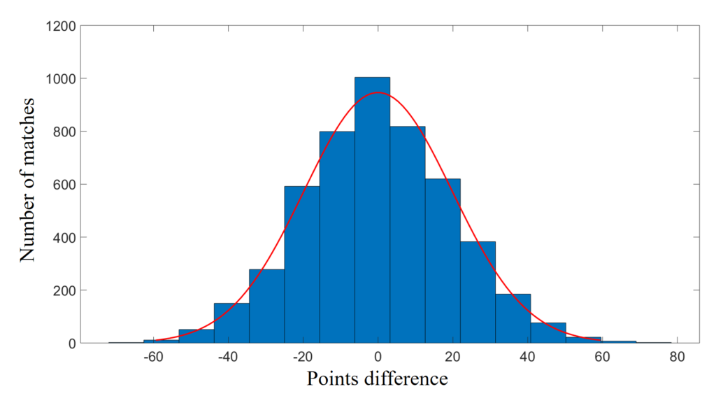
Let’s start by having a look at the missed tackle differential between the teams (home team missed tackles minus away team missed tackles), just as we looked at the points differential in the previous post.

We expect the mean missed tackle differential between two evenly matched sides to be zero. For our 5000 Monte Carlo simulations the mean was -0.1 with a standard deviation of 9.1. This mean is more than close enough to zero for our purposes, and we note that if we had carried out more simulations this value would have eventually converged in zero.

What would we expect the mean and standard deviation of the missed tackles of a real rugby competition to be, based on this result? Well we might expect the mean to be a little less than zero if the missed tackles are somehow involved in the hometeam advantage seen in part I, and the home team misses less tackles than the away team. We might also expect that the standard deviation will be larger since in a real competition not all matches will be played between such closely matched teams. This will result is a larger spread in missed tackles as the result of a larger skill differential between the sides, and hence a larger standard deviation. The mean and standard deviation of the missed tackle differential in the 2016 Super Rugby competition was -3.0 with a standard deviation of 11.2. As hypothesised, the mean is a little less than our simulations and the standard deviation larger, and this gives us some degree of confidence that things are as they should be.

Returning to the simulation results, by tallying up the simulation results we produce the table below which shows the probability of various missed tackle differentials from the perspective of the home team.

Probability of missing less and more tackles than the opposition for two evenly matched teams.

Result	Probability (%)
15+ less missed tackles than opposition	4.3
11 to 15 less missed tackles than opposition	8.5
6 to 10 less missed tackles than opposition	15.0
1 to 5 less missed tackles than opposition	21.1
Misses tackles equal to opposition	4.5
1 to 5 more missed tackles than opposition	20.1
6 to 10 more missed tackles than opposition	14.3
11 to 15 more missed tackles than opposition	7.6
15+ more missed tackles than opposition	4.6

Let’s say that in a given match a team misses 6 more tackles than their opposition. Summing the bottom three rows of the table shows us they should expect to do this by chance 14.3 + 7.6 + 4.6 = 26.5 % of the time.

For arguments sake we’ll assume missing 6 or more tackles than our opposition would result in the coach berating his players for their poor defensive commitment and putting them through a defense focused training regime the following week, at the expense of time spent on other areas of training (since there is only so much training time available).

Is this an unjustified decision by the coach? Well, if the coach has no other valid reason to believe his defense has suddenly become worse, then it is absolutely an unjustified decision.

And this is where many people get into trouble with their thinking when making decisions like this. Their argument goes something like, ‘they defended poorly, therefore they need to train defense’. However, they only defended poorly in the misguided sense that it was not the result we hoped for. In reality, this is just a legitimate sample from the teams performance profile, or distribution of outcomes. No team or individual should be berated for producing expected samples from their distribution. To do so is nonsensical, just as it would be nonsensical to berate a coin for producing a head when we were hoping for a tail.

To try and understand this better let’s drill down a little further by looking at the individual performances in a single game where the home team missed 6 more tackles than their opposition. The table below shows the players who missed tackles in a single such game, and therefore contributed to the 6 more tackles missed than the opposition in this particular game.

Players who missed tackles on the home team in a single match in which the home team missed 6 more tackles than the away team

Position	Missed tackles
Prop	3
Openside flanker	3
Number eight	3
Hooker	2
Prop	2
Blindside flanker	2
Wing	2
Outside center	2
Lock	1
Halfback	1
Inside center	1
Fullback	1

The table shows that 12 players contributed to a total of 23 missed tackles. The average missed tackles per game for a side in the 2016 Super Rugby contest was about 20, so this team missed 3 more than average. Because we know that they missed 6 more than their opposition in this particular game, we know that the opposition must have missed three less tackles than average. The worst offenders were three players who each missed three tackles each. Let’s pick on the first player listed in the table, the prop who missed three tackles, by examining his performances a little more closely. We’ll do this by looking at the his missed tackle performance profile as represented by the probabilities in the table below calculated over the 5000 Monte Carlo simulations for which we have data on him.

Single game missed tackle probabilities calculated from 5000 Monte Carlo match simulations for the prop (jersey number 1) on the home team.

Number of missed tackles	Probability (%)
0	35.0
1	35.3
2	18.9
3	7.1
4+	3.6

The table shows us that our prop is normally a pretty reliable performer missing 0 or 1 tackles in more than 70% of the matches he plays. He will miss 3 or more tackles 7.1 + 3.6 = 10.7 % of the time. So whilst the 3 tackles he missed in the particular match above are not his usual performance, they still constitute expected results from his performance distribution. Therefore, unless we have other any valid reasons to believe he might be getting worse at tackling we should probably just except that this is the result of chance. Approaching him when there is no valid reason to do so may put unnecessary strain on the player coach relationship. If he missed say 4 or more tackles in consecutive games we might be more justified in taking some action since this would only be expected to happen 0.1 % of the time (0.036 x 0.036 x 100).

As a side note it will generally be better to monitor the proportion of successful skill executions. In the case of missed tackles this would be the number of missed tackles divided by the total tackles attempted. But that is a story for another day, and does not change the point we are trying to illustrate here.

So what should you do if you want to improve your teams tackling? Obviously you should train tackling. All we are saying here is that you should not make the decision to prioritise this training based on a flawed reactive understanding of probability. We’ve all seen teams who do this. One week they need to fix their defense. The next their defense is fixed but their handling needs work. Then they aren’t fit enough. Then the defense they miraculously fixed a few weeks back, has somehow broken again, and the cycle continues. This headless chook approach to coaching is a pretty good sign of a coach with no understanding of probability. Don’t be surprised to see their team sitting closer to the bottom of the ladder.

A team that can avoid this approach, will have a better chance of getting their training priorities right just by virtue of the fact they will be less likely to overcommit training time to certain areas, and as a result neglect others. In the long term they will gain advantage over other teams employing the headless chook approach.

Just what training priorities should be is another question all together. Naturally we should focus on those things that contribute the most to winning. But what are those? How do they differ for different teams? Those are questions we will look to answer in a future article.

Finally bare in mind that although this article has used tackling as an example, the general principles obviously apply to anything we might consider training. Bare in mind also that training players in a skill will result in their distribution or performance profile for that skill changing. This then becomes the new standard which they should be evaluated against when determining whether or not their is any reason to be concerned about their recent performances.

Bounce of the ball. Rub of the green. Chance. Whatever you want to call it, we all know it plays some kind of role in determining the outcome of our favourite sporting contests. But just how important is it? That’s the question we will answer in this article for a rugby match between two evenly matched teams.

If we think about two evenly matched teams, we all intuitively understand that each team will win 50% of the time. We don’t need any sophisticated math to tell us this. It’s a simple coin flip.

Most of us also assume that a match between two perfectly evenly matched sides will be close. But is this true? How close is close?

It’s an important question to answer, simply because the careers of coaches and players hinge on wins and losses. A big loss, or series of losses, often sees coaches fired and players dropped. On the other hand, a big win or series of wins might be enough to earn a coach or player a new contract.

Once again, we can use Monte Carlo simulation to shed light on this situation. For those looking for a brief introduction to how we are using Monte Carlo methods in a sporting context, have a read of the first post where we considered how good a rugby team where the great Jonah Lomu occupied every position might be. But for now, we’ll get right to it and carry out 5000 full rugby match simulations between two evenly matched sides playing at the professional club level.

What do we expect the mean points differential (home team score minus away team score) between the sides to be?

In the absence of any home team advantage, which our simulations assume, the answer is zero. The points difference between two evenly matched sides should always average out to zero in the long term. The mean of our 5000 Monte Carlo simulations is just that, 0.0.

The standard deviation of the points differences of our simulations is 19.8. For those not familiar with statistics, the standard deviation simply tells us how much our data is spread out around the mean. The higher the value the more it is spread away from the mean. In the case of points difference, a higher standard deviation means more games are won and lost by large margins. A lower standard deviation means more games are won or lost in closely contested matches.

What would we expect the mean and standard deviation of a real rugby competition to be based on this result? Well, we would expect the mean to be a little more than 0 (we are talking from the perspective of the home team), since home town advantage is generally considered to be a real phenomenon. We would also expect the standard deviation to be a little more than 19.8, since in real professional competitions not all games are played by evenly matched teams. When two teams meet where one is a better than the other we would expect the points differential to be on average a little more, and therefore the spread in our data, as indicated by the standard deviation, to be a little more.

The mean of the points differential of games from the 135 round robin games played in the 2016 Super Rugby contest was 4.3 with a standard deviation of 21.9. As we hypothesised, the mean and standard deviation of the real world competition are a little larger than what our Monte Carlo simulations predict for two perfectly evenly matched teams. This comparison gives us some degree of confidence in the output of our simulations.

As a side note, the difference between the mean points difference of our simulations and that of the Super Rugby data is statistically significant, which suggests home team advantage is real and worth about 4 points per game. Note also, that the distribution of points differences is also approximately normal. This is quite a useful result, but not essential to what we are trying to do here so I have discussed this a little more at the end of the article.

Let’s get back to our main objective of determining how important chance is in determining the outcome of rugby games.

We are interested in the percentage of games that fall into any given score category. We can calculate this simply by counting up how many games fall into say the win by 1 to 10 points category (from the perspective of the home team in our case). These results are shown in the table below.

Probability of losing and winning a rugby match by various margins for two evenly matched teams.

Result	Probability (%)
Loss 30+	6.4
Loss 21 to 30	8.8
Loss 11 to 20	14.4
Loss 1 to 10	19.1
Draw	3.0
Win 1 to 10	19.0
Win 11 to 20	14.1
Win 21 to 30	8.7
Win 30+	6.5

What struck me immediately is the first entry in the table, which shows we will lose around 6.4% of games by more than 30 points. So, against a team who is our equal, chance will have us get absolutely flogged about 1 in every 15 times we meet. A 30 point drubbing is the sort of result that has fans baying for blood, and starts to make coaches feel nervous. Especially when everyone was expecting a close game against an evenly matched opponent.

What about close games, how often will we actually get them? For the purposes of this discussion we’ll consider a close game to be a win or loss by 10 or less, or a draw. The table shows that this will happen about 19.1 + 3.0 + 19.0 = 41.1 % of the time. So rather than being the norm, a close result is actually in the minority of results.

The table also shows that a given team will suffer a relatively heavy loss by 11 or more points 14.4 + 8.8 + 6.4 = 29.6% of the time. For arguments sake, let’s assume that two such losses in a row would be enough for the clubs fans and administrators to start asking some serious questions about the quality of their coaching staff and players. Through chance alone, the probability of this happening in the next two games the team plays is about 8.8 % (0.296 x 0.296 x 100).

Let’s assume that after three such losses the club has had enough and they start looking at new coaching options for next season. Or perhaps one or two particular players happened to perform poorly in a couple of those matches, and the club starts looking to move them to another club. Through chance alone, the probability of this happening in the next three games the team plays is about 2.6 % (0.296 x 0.296 x 0.296 x 100).

What this tells us is that a team that does not understand probability, will be prone to making some terrible operational decisions. This in turn creates opportunities for those who do understand probability.

If one team can spot another team who has fallen into the above situation, and is looking to shed coaches and/or players when there are no other valid reasons to believe these coaches or players have suddenly become worse, then there will be an opportunity to recruit them to their own club which may not have otherwise existed. Even better, they will likely be available at a discount rate.

Of course, there will be times when there are problems at a sporting organisation. We can use an understanding of probability to help detect these too. As a simple example, the probability of suffering two losses by more than 30 points in a row for our evenly matched sides would be only 0.4 % (0.064 x 0.064 x 100). Because this is very low, if it were to happen in real life it would probably be worth investigating if there are any reasons that might have led to this. If it is indeed an outlier, we might be able to find another underlying event or circumstance that is also out of the ordinary that led to this. Perhaps one player had an exceptionally poor game, and on further investigation we find out that there was an underlying injury we were not aware of, or even or personal issue. Perhaps the player is aging and this is a trigger for us to start closely monitoring his typical performance profile to see if it is declining. The list goes on, but the point is an understanding of probability can be used to our advantage as an indicator of when to invest time digging deeper into events, and when to leave them be.

In summary, we have seen that the bounce of the ball in the form chance has a surprisingly large impact on the outcome of a rugby game, even when two teams are evenly matched. We’ve also seen that a team that understands this can exploit it to their advantage by recruiting coaches and players from other teams who have discarded them in error (and equally by not unfairly discarding coaches or players from their own side). They can also use an understanding of probability to try and detect when there may well be problems in their organisation.

That’s not the end of the story though. In part two of this article we will look at how teams can explore the same concept to try and avoid getting their training priorities wrong.

Some notes on normality

Earlier in this article it was stated that the distribution of points differentials of our Monte Carlo simulations turns out to be well approximated by a normal distribution. This can be seen in the nice bell shape in the histogram below.

We shouldn’t always expect populations to be normally distributed. But when they are we can use standard normal distribution calculations to easily calculate any probability we are interested in. The table below compares the Monte Carlo calculated probabilities from earlier with those calculated under the approximation of a normal distribution. We can see that the two agree very closely.

Probability of losing and winning a rugby match by various margins for two evenly matched teams. As calculated from 5000 Monte Carlo simulations (column 1) and predicted from standard normal distribution calculations (column 2) using a mean of 0 and standard deviation of 19.8.

Result	Probability (%)	Probability (% predicted)
Loss 30+	6.4	6.2
Loss 21 to 30	8.8	8.9
Loss 11 to 20	14.4	14.8
Loss 1 to 10	19.1	19.2
Draw	3.0	2.0
Win 1 to 10	19.0	19.2
Win 11 to 20	14.1	14.8
Win 21 to 30	8.7	8.9
Win 30+	6.5	6.2

Being able to use standard normal distribution calculations not only gives us the ability to calculate any probability we are interested in easily, but has the advantage of being able to do so without having to iterate through or even have access to the simulation results. For example, if you know how to carry out such calculations you can verify that the probability of winning a game by 13 or more for two evenly matched sides is about 26 % and by 40 or more about 2 %.

In this first article we pay homage to the late great Jonah Lomu by attempting to use Artificial Intelligence (AI) to answer the question of how good a rugby team where Jonah Lomu played every position would be.

The most successfully used AI technique for making decisions in games are Monte Carlo algorithms. These have been applied to achieve human level performance in games such as Go and Chess.

We’ll begin here with a brief explanation of how a Monte Carlo algorithm can be applied in the context of replicating player decision making in sport. In future articles we will layer in further details on how these and other AI and mathematical techniques work, and how they can be used to assist in making decisions in sporting operations.

To utilise a Monte Carlo algorithm in a full match rugby simulation we must first build a model of the sport which describes the physical environment and the rules of play. Armed with this, we need to allow players within the environment to make decisions, for better or worse. Consider a virtual rugby player standing in such an environment carrying the ball and faced with the decision to run left, right, straight, or pass to the player next to him. Depending on the player we might allow him to consider many more decisions such as other passing options, fending off a defender, or a chip kick over the defence. In a Monte Carlo algorithm we allow the player to effectively simulate each of his options, perhaps many times each. The player is effectively thinking through his options and considering their outcomes. He then chooses the option to take based on the outcome or average outcome of these simulations relative to his objectives and what he perceives to be important.

Combining the model of the physical environment, rules of play and decision making process we effectively end up with what could be termed an AI engine capable of modelling a sport. We’ve spent the past few years developing such an engine for the sport of rugby, and we will be using it here and in coming articles to answer many questions about the sport of rugby, but the results and approach will often be generally applicable to many sports.

Once we have an engine/model, we can use it to answer a question by performing Monte Carlo simulations of entire matches or parts of them (as differentiated from the Monte Carlo decision making algorithm discussed above). A simple way to understand Monte Carlo simulation of a match is to imagine rolling a six sided die 10,000 times and recording the result of each roll. If you did this you would be able to get a reasonably accurate estimation of the probability of a 6 being rolled which would be close to the true value of 1/6. What say you then weighted one of the sides? You could then re-run the experiment rolling the die another 10,000 times and determine what effect this weight had on the probability of rolling a 6, something that might be very difficult to determine otherwise.

This is the exact same approach we will use here, except in our case the AI engine is the die and the outcome is the result of the match and all the data that comes along with it (e.g. points scored, tackles made etc.). We’ll perform many simulations with standard players and then many simulations when each of the players are progressively replaced by someone with the key attributes of Jonah Lomu. From the difference we will be able to answer our question of how good a team of Jonah Lomu’s would be.

In our case, our standard players have attributes (speed, acceleration, handling error probability, tackle success probability etc.) taken from various sources which describe typical rugby players (with positional specificity where available) at about the level of a current professional club player. Using these players as our input, the AI engine and the assumptions it are based on have been adjusted until the output matches that of the Super Rugby competition. This process of modelling and model validation is very important and something we will detail further in future articles. For now, we will just accept that we are satisfied with the results of this process, so that our next task is to ask what should the input attributes of Jonah Lomu be?

To make things simpler we will consider the attributes which perhaps contributed most to Jonah’s ability to terrorise his opposition: height, weight, speed, acceleration, and of course, his ability to break tackles. In all other attributes we will consider him the equal of the typical player in each position. For example, we’ll assume the front row version of Jonah can scrummage and the flyhalf version is adept at kicking for touch.

With that in mind, Jonah was about 120 $latex kg &s=0$ and 1.96 $latex m &s=0$ tall. He was exceptionally fast for a man of his size and able to run the 100 $latex m &s=0$ sprint in 10.8 $latex s &s=0$ in his prime. If we assume his acceleration was about that of a typical rugby back at 6.31 $latex m.s^{-2} &s=0$ then his maximum speed can be calculated as 9.99 $latex m.s^{-1} &s=0$. Imagine that, the big man storming toward you covering around 10 meters every second. Not an easy prospect for a defender.

As a side note, it’s implicit in the above that we are assuming rugby players can be adequately described as accelerating constantly to maximum speed. This is an example of one of the many simplifying assumptions made in our AI engine which help to ensure our Monte Carlo approach remains computationally feasible in a reasonable amount of time. We’ll detail other assumptions as they arise in future articles. Given adequate data, we can often demonstrate the validity of such simplifying assumptions by showing that they have negligible impact on the output we are interested in.

Finally, in the absence of any hard data we will assume the probability that Jonah would break a tackle was twice that of a typical player. It’s probably a fair estimate. Just ask the English fullback Mike Catt who was trampled by Jonah on his way to score a try in the 1995 Rugby World Cup quarter final between New Zealand and England.

Having estimated our input data for Jonah Lomu, we are now ready to carry out our simulations. Rather than just replace the entire team at once, we’ll replace them one by one in the following order by jersey number 11, 14, 15, 13, 12, 10, 9, 8, 7, 6, 5, 4, 3, 2, 1. For those not familiar with rugby this amounts to replacing the outside backs (11, 14, 15) followed by the remaining backs (13, 12, 10, 9) and finally the forwards. Backs are generally faster and more agile players who look to exploit space and finish scoring opportunities. Forwards are generally bigger and stronger and are crucial to controlling and maintaining possession of the ball on attack.

Jonah was a winger and wore jersey 11, so we are replacing his position first. The graph below shows the effect of sequential replacement of each player on the team by Jonah on the winning percentage of the team. Each data point represents 2000 match simulations.

When zero players are replaced (our control) the win percentage is around 50%, representing a match between two identically matched sides. The winning percentage is actually slightly lower than 50% as a result of draws. It turns out that draws account for around 3% of all results when teams are perfectly evenly matched. This number reduces to much less than 1% as teams become increasingly mismatched.

Replacing just one player in Jonah’s 11 jersey results in only a small increase in winning percentage. This obviously shows that one man can’t make a team, especially in a 15 aside game like rugby union. But it is perhaps also a tribute to Jonah and the impact he had on the sport of rugby. Before Jonah came along rugby union wingers were generally smaller. In the modern game there are plenty of big wingers, and that change is at least partly attributable to Jonah Lomu demonstrating how devastating a big fast man on the wing can be. So because our baseline player attributes are that of a modern winger, replacing them with Jonah has a small but not drastic effect. Smaller than it would have been back when Jonah burst onto the world rugby stage in the mid 90’s.

However, as we progress through the rest of the backline replacing each player with Jonah Lomu like players as we go, the effect of winning percentage starts to increase drastically, reaching about 85% once the entire backline has been replaced. It is clear that an entire backline with all their position specific skills in tact, and yet still sporting the size and mobility of Jonah would be fairly unstoppable, and certainly not something the modern game has ever seen. Though, with player sizes seeming to continue to trend upward, it is something we might see in the future!

As we continue through the forwards the winning percentage continues to climb, before leveling out as it reaches more than 99% by the time the locks have been replaced. We barely even need to bother replacing the final three players in the front row of the forward pack, as the damage is already done. Although modern forwards are of similar size to Jonah Lomu, once they are endowed with his speed and acceleration as they have been here, they become virtually unstoppable.

When all is said and done the final winning percentage once all 15 players have been replaced is 99.8%. So, we have answered our initial question. A team where every player possesses the physical characteristics of Jonah Lomu, whilst retaining the skills specific to their position would be almost impossible to beat.

As an interesting side note, the classic video game ‘Jonah Lomu Rugby’ released in 1997 featured an unlockable ‘Team Lomu’ which had Jonah in every position. Just as we predicted here, they were pretty unstoppable!

Although the subject of this article has considered a hypothetical scenario, it points to more practically useful applications of AI in sports. Things like determining what we should train players in, and who we should recruit.

In essence, all applications boil down to potentially allowing us to determine what is important to winning. We will explore such applications in the future and try to answer questions like,

What makes the All Blacks so good?

How important are offloads in the modern game of rugby?

What are the most important physical attributes and skills to train?

Would recruiting Usain Bolt be a good idea for a rugby team?

What is the effect of a bad refereeing call?

In the next article we will determine how important the bounce of the ball is in determining the result of a rugby match.